A Simple Ocean Data Assimilation retrospective analysis of the global ocean 1950-1995
James A. Carton*, Gennady Chepurin*, Xianhe Cao*, and Benjamin Giese**
January 18, 1998
submitted to the Journal of Physical Oceanography
*Department of Meteorology, University
of Maryland, College Park, MD 20742
**Department of Oceanography, Texas
A&M University, College Station,
TX
Abstract
We describe a 46-year global retrospective analysis of upper ocean temperature, salinity, and currents. The analysis is an application of the Simple Ocean Data Assimilation (SODA) package. SODA uses an ocean model based on Geophysical Fluid Dynamics MOM2 physics. Assimilated data includes temperature and salinity profiles from the World Ocean Atlas-94 (MBT, XBT, CTD, and station data), additional hydrography, sea surface temperature, and altimeter sea level.
After reviewing the basic methodology we present experiments to examine the impact of model forecast bias and trends in the wind field. We believe these to be the major sources of error in our retrospective analysis. Additional experiments examine the relative importance of winds versus subsurface updating. These experiments show that in the tropics both winds and subsurface updating contribute to analysis temperature, while in midlatitudes the variability results mainly from the effects of subsurface updating.
Finally, we present a simple examination
of variance. We separate the analysis into four frequency bands, annual,
interannual (1 - 5 yr), decadal (5 - 25 yr), and the long-term trend. At
the annual frequency the results confirm previous results regarding the
response of the ocean to seasonal winds and heating. In the interannual
band, the most prominent signal in the temperature field is associated
with El ![]() Oscillation. Although
this mode is focused in the tropical Pacific, we can identify global structure.
In the decadal band we discuss a basin-scale mode in the North Pacific
Ocean that has been associated with the Pacific-North America pattern of
wind variability, while in the North Atlantic we discuss a basin-scale
mode that has been associated with the North American Oscillation pattern
of wind variability. The long-term trend of heat content reveals a pattern
of warming in the subtropics and cooling in the tropics and at high latitude.
Oscillation. Although
this mode is focused in the tropical Pacific, we can identify global structure.
In the decadal band we discuss a basin-scale mode in the North Pacific
Ocean that has been associated with the Pacific-North America pattern of
wind variability, while in the North Atlantic we discuss a basin-scale
mode that has been associated with the North American Oscillation pattern
of wind variability. The long-term trend of heat content reveals a pattern
of warming in the subtropics and cooling in the tropics and at high latitude.
1. Introduction
In this paper we describe the Simple Ocean Data Assimilation (SODA) package and its application to the construction of a retrospective analysis of the ocean. Our goals are twofold, first to develop software to explore some of the technical aspects of data assimilation, and secondly, to construct a long, nearly fifty year retrospective analysis of the temperature, salinity, and circulation of the upper layers of the ocean for use in climate studies. The historical set of observations is far too limited to allow such a reconstruction alone, without additional assumptions. Several previous attempts have been made to reconstruct basin-scale historical changes in the ocean. This retrospective analysis differs from previous analyses (White, 1995; Levitus, et al., 1994; Rosati, et al., 1995; Smith, 1995; Ji et al., 1995) by its global spatial scale, multi-decadal temporal scale, and by the relative sophistication of the assimilation algorithms.
Still, in developing this package we have attempted to choose simplicity over innovation where possible. The general circulation ocean model on which the analysis is based uses the Geophysical Fluid Dynamics Laboratory Modular Ocean Model 2.b code, with conventional choices for mixing, etc. The constraint algorithm we apply is an extension of optimal interpolation, an algorithm that has been widely applied in meteorological numerical weather forecasting. Our extension includes changes in the spatial dependence of the statistics, and in the assumption of bias in the model forecast. Still, our approach is less sophisticated than the computationally intensive Kalman Filter which predicts the temporal and spatial evolution of the error statistics. Optimal interpolation bears a close similarity to variational methods as well, when the constraint being minimized is the mean square error. A comprehensive discussion of the alternatives is provided by Bennett (1990), Wunsch (1996), and Malanotte-Rizzoli (1996).
The domain of this analysis extends from![]() .
The main data sets used to constrain the model are the hydrographic data
contained in the World Ocean Atlas 1994 (WOA-94
Levitus and Boyer, 1994), additional hydrographic data, satellite
and in situ sea surface temperature (Reynolds
and Smith, 1994), and altimetry from the Geosat, ERS1, and TOPEX/Poseidon
satellites. The historical data set is sufficiently limited that we have
made no attempt to resolve midlatitude mesoscale variability and have limited
our attention to the upper 500m of the water column. Most analysis experiments
begin January, 1950 and continue through December, 1995. The basic analysis
fields consist of 552 monthly averages of temperature, salinity, and the
horizontal components of velocity. In order to simplify presentation of
the results most of the discussion in this paper focuses on heat content,
defined as the vertical integral of temperature 0/500 m.
.
The main data sets used to constrain the model are the hydrographic data
contained in the World Ocean Atlas 1994 (WOA-94
Levitus and Boyer, 1994), additional hydrographic data, satellite
and in situ sea surface temperature (Reynolds
and Smith, 1994), and altimetry from the Geosat, ERS1, and TOPEX/Poseidon
satellites. The historical data set is sufficiently limited that we have
made no attempt to resolve midlatitude mesoscale variability and have limited
our attention to the upper 500m of the water column. Most analysis experiments
begin January, 1950 and continue through December, 1995. The basic analysis
fields consist of 552 monthly averages of temperature, salinity, and the
horizontal components of velocity. In order to simplify presentation of
the results most of the discussion in this paper focuses on heat content,
defined as the vertical integral of temperature 0/500 m.
In an companion study Carton
et al (1998) examine the accuracy of the SODA analysis by comparison
to a variety of independent observations. The independent observations
include tide gauge sea level, altimeter sea level (when it is excluded
from the updating data set), hydrographic sections, station temperature
and salinity time series, surface drifters, and moored currents. In summary,
these comparisons show that the analysis explains 25-30% of the observed
tide gauge sea level variance at longer than annual frequencies. The root-mean-square
difference of observed minus analysis sea level in the tropics (![]() )
lies in the range of 3.1-4.0 cm, increasing somewhat in midlatitudes. The
comparison at ocean weather station S near Bermuda as well as comparison
to independent hydrographic transects point to the importance of bias in
the forecast model as a major source of error in the analysis.
)
lies in the range of 3.1-4.0 cm, increasing somewhat in midlatitudes. The
comparison at ocean weather station S near Bermuda as well as comparison
to independent hydrographic transects point to the importance of bias in
the forecast model as a major source of error in the analysis.
Forecast bias results from the fact that general circulation models develop climatologies that differ from the true climatological state (the problem of bias in meteorological models is described in Thiebaux and Morone, 1990). There are several causes of forecast bias: insufficient resolution, inadequate modeling of unresolved physics, and biases in surface forcing fields of wind, heat, and freshwater. Most implementations of the constraint algorithms listed above assume, for convenience, that the error statistics are unbiased. To understand the impact of this unfortunate assumption we examine the change in the analysis that happens when this assumption is eliminated (Expt. 1 in Table 1).
The remainder of this paper examines the variability of the analysis. The source of variability of heat content is identified by comparison to a set of three experiments. Because the forcing fields and the dynamics of the ocean vary with frequency we decompose the results into four bands, annual, interannual, decadal, and the long-term trend. These results are presented in Section 4.
Table 1. Ocean analysis experiments presented in the text. Each experiment covers the period 1950-1996.
2. Data
In the period before the mid-1980s the main data sets we have to provide constraints on the subsurface density field are profile measurements of temperature from mechanical bathythermograph (MBT), expendable bathythermograph (XBT), conductivity-temperature-depth (CTD), measurements from thermistors and reversing thermometers, and salinity from CTD and station measurements. Since late-1986 satellite altimetry has added an additional powerful constraint on column-averaged density. However, even during this later period subsurface measurements are required in order to determine the vertical distribution of density variations implied by the altimetry. The sources of these data are described below.
Hydrography
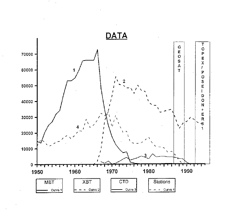
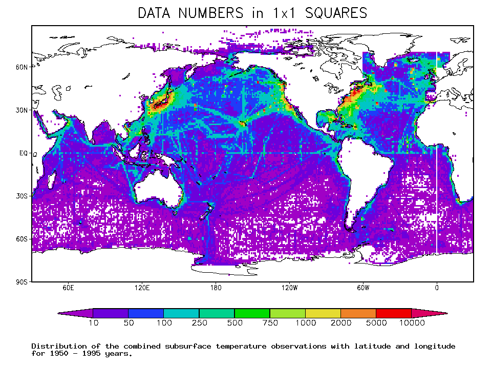
We began with the data sets contained in WOA-94. From WOA-94 we extracted temperature and salinity data records obtained by four different instrument types: MBTs, XBTs, CTDs and salinity-temperature-depth probes (listed combined as CTDs), and station data. The temporal distribution of the data sets is shown in Fig. 1a. Until the late-1960s MBTs provide the majority of upper ocean temperature profiles, while stations provide the majority of salinity and temperature measurements below 200m. After 1968 XBTs replace MBTs as the major data set, while the number of station observations begins to fall off. The change to XBTs means a substantial increase in data between 200m and 450m as well. The spatial coverage of the subsurface temperature data is presented in Fig. 1b. The observations are mainly limited to the Northern Hemisphere, and are concentrated along commercial shipping routes.
The error characteristics of the instruments vary widely. The MBT and XBT instruments infer depth from drop-rate and thus are subject to random and systematic errors that increase with depth (the random error is generally assumed to be 1-2% of depth). Systematic errors in the drop-rate of XBTs depend on the type, and even the batch of the XBT. Here we have applied the empirical corrections of Levitus and Boyer (1994) to try to limit this source of bias.
The data contained in WOA-94 is limited mainly to the years prior to 1991. We have supplemented this with data from the XBT archive of the National Oceanographic Data Center and the Coupled Modeling Project of the NOAA National Center for Environmental Prediction (NCEP). We have also included temperature data produced by the Tropical Ocean Global Atmosphere Tropical Atmosphere-Ocean (TOGA/TAO) moored thermistor array. Additional data is provided by a variety of research programs, including, for example, the Soviet SECTIONS tropical program, and the Western Tropical Atlantic Experiment. Data from the World Ocean Circulation Experiment hydrographic surveys has been withheld to provide independent comparison (Carton et al., 1998).
With such a wide variety of data sets, quality control becomes extremely important. Much of the combined data set was checked prior to entry into WOA-94. We found it useful to complete our own additional checks for duplicate reports and errors in the recorded position and time of observations. We also check each profile for vertical stability, and for the extent of its deviation from climatology, including the relationship between temperature and salinity. Observations differing from climatology by more than three standard deviations were assumed to be in error and thus were excluded. Altogether these data checks eliminated approximately 10% of the data. Of the criteria we applied, the most restrictive was the comparison to climatology. We believe the most serious problems with the in situ observations result from mistakes in station location reports.
The analysis is carried out at each of
the model levels between the surface and 443.79 m. The profile data is
interpolated onto these model levels using a quadratic interpolation procedure
(profiles were eliminated if the vertical resolution was insufficient).
The main reason for this limitation is the lack of data at deeper model
levels. After vertical interpolation the temperature observations were
binned into ![]() bins. The resulting
super-observations form the basic temperature and salinity data
sets used in this study.
bins. The resulting
super-observations form the basic temperature and salinity data
sets used in this study.
Altimetry
The altimetry used in this study is the
Pathfinder Project version 2.1 and has been obtained from the Pathfinder
web site. The altimetry comes from four different instruments flying on
GEOSAT, ERS/1, and the TOPEX/POSEIDON platforms. The orbital characteristics
of the altimeters are described in Table
2. Each instrument and platform requires independent calibration
procedures, most of which were carried out as part of the Pathfinder processing.
We have added the usual corrections for geophysical effects, and then averaged
sea level estimates into ![]() latitude
segments. The once-per-revolution harmonic has been removed from the Geosat
altimetry because of contamination by planetary-scale error. No additional
filtering or interpolation has been performed.
latitude
segments. The once-per-revolution harmonic has been removed from the Geosat
altimetry because of contamination by planetary-scale error. No additional
filtering or interpolation has been performed.
Table 2 Satellite altimetry used in this study
| Satellite | Days/Repeat cycle | Revolutions/Repeat cycle | Span of Data |
| GEOSAT ERM | 17.05 | 244 | 11/8/86 - 9/30/89 |
| ERS1 (35dy repeat) | 35.00 | 501 | 4/14/92 - 12/20/93 |
| TOPEX/POSEIDON | 9.92 | 127 | 9/30/92 - 11/28/96 |
3. Analysis methodology
3.1 Assimilation methodology
In this section we briefly describe our
estimation algorithm and associated statistical models. The theoretical
basis for optimal interpolation is described in Daley
(1991), while extensions to account for bias in the forecast model
are described in Dee and da Silva (1997).
We begin by assuming that a forecast ![]() ,
exists at time
,
exists at time ![]() . Here
. Here ![]() is
a state vector containing all model variables at each grid-point.
is
a state vector containing all model variables at each grid-point. ![]() is
provided by integration of a model based on initial conditions at time
is
provided by integration of a model based on initial conditions at time
![]() . We assume
. We assume ![]() differs
from the 'true' state
differs
from the 'true' state ![]() due to
the presence of model bias,
due to
the presence of model bias, ![]() ,
and random Gaussian distributed forecast error,
,
and random Gaussian distributed forecast error, ![]() .
.
![]() (1)
(1)
The quantity in parentheses is referred
to as the bias-corrected forecast: ![]() .
Throughout this discussion we use a tilde to indicate a bias-corrected
variable. All observations (of temperature, salinity, sea level, etc.)
are collected into an observation vector
.
Throughout this discussion we use a tilde to indicate a bias-corrected
variable. All observations (of temperature, salinity, sea level, etc.)
are collected into an observation vector ![]() of length
of length ![]() at time
at time ![]() .
We define the observation error,
.
We define the observation error,![]() ,
to be the difference between the observed and true state interpolated
to the observation location
,
to be the difference between the observed and true state interpolated
to the observation location![]() -
-![]() .
. ![]() includes
measurement error, error of representativeness, and error due to unresolved
physics.
includes
measurement error, error of representativeness, and error due to unresolved
physics. ![]() is the interpolation
operator which maps the analysis variable type into the observation variable
type at the observation location and time. We immediately approximate this
equation as
is the interpolation
operator which maps the analysis variable type into the observation variable
type at the observation location and time. We immediately approximate this
equation as
![]() -
-![]()
where  .
Now we summarize the analysis equations. Minimizing the mean square
error leads to the interpolation equation for the analysis
.
Now we summarize the analysis equations. Minimizing the mean square
error leads to the interpolation equation for the analysis
![]() (2)
(2)
The forecast bias is assumed to be slowly
evolving with time. We can anticipate, for example, that there will be
a substantial seasonal dependence to the bias. The certainty with which
we know the bias deteriorates even more rapidly with time. To account for
these time-dependencies we will use as our first guess of the bias at ![]() a fraction of the bias at the previous update time (in this study, 10 days
earlier).
a fraction of the bias at the previous update time (in this study, 10 days
earlier).
![]() (3)
(3)
After examining the results of a few experiments
we have chosen a value of ![]() ,
making the first guess of the bias decay with a time scale of roughly 20
days. We begin at
,
making the first guess of the bias decay with a time scale of roughly 20
days. We begin at ![]() by assuming
zero bias. The bias is updated using equations similar to the analysis
equation
by assuming
zero bias. The bias is updated using equations similar to the analysis
equation
![]() (4)
(4)
The gain matrices ![]() and
and ![]() depend on the forecast,
observation, and bias error covariances
depend on the forecast,
observation, and bias error covariances
![]()
as:
![]() (5a)
(5a)
![]() (5b)
(5b)
The parameter ![]() determines what part of the total error is random and what part is due
to bias. A value of zero corresponds to the assumption that all error is
random, whereas a value of one corresponds to the assumption that all error
is due to bias. For the sake of computational efficiency (5a,b) are currently
solved locally in a series of patches spanning 25 horizontal grid-points
each. The global solution is then constructed by assembling the patches.
determines what part of the total error is random and what part is due
to bias. A value of zero corresponds to the assumption that all error is
random, whereas a value of one corresponds to the assumption that all error
is due to bias. For the sake of computational efficiency (5a,b) are currently
solved locally in a series of patches spanning 25 horizontal grid-points
each. The global solution is then constructed by assembling the patches.
In the control analysis we choose the usual
assumption of no bias and set![]() The dependence on this assumption is examined in Expt.
1. In this experiment we assume
The dependence on this assumption is examined in Expt.
1. In this experiment we assume ![]() following the recommendation of Dee and
da Silva (1997) based on studies with a shallow water model.
The effect of assuming the existence of bias is for the analysis fields
to be shifted in regions of high data coverage to correct for forecast
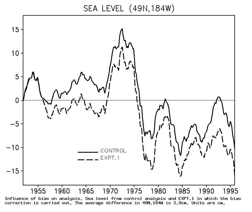
bias. The effect of the bias correction on the analysis in the central
basin is illustrated in Fig. 2 at
a point in the central North Pacific (
following the recommendation of Dee and
da Silva (1997) based on studies with a shallow water model.
The effect of assuming the existence of bias is for the analysis fields
to be shifted in regions of high data coverage to correct for forecast
bias. The effect of the bias correction on the analysis in the central
basin is illustrated in Fig. 2 at
a point in the central North Pacific (![]() ).
Here the bias correction algorithm has the effect of lowering the analysis
sea level by about 2-4 cm. The drop in sea level is mainly the result of
an elevation of the thermocline by varying amounts of up to 20 m.
).
Here the bias correction algorithm has the effect of lowering the analysis
sea level by about 2-4 cm. The drop in sea level is mainly the result of
an elevation of the thermocline by varying amounts of up to 20 m.
The effect on temperature and salinity
accuracy of the bias correction algorithm can be examined by comparing
the control analysis and Expt. 1
with observations at Ocean Station S in the northwest Atlantic (![]() ).
At this station the impact of the bias correction at 443m (within the thermostaad)
is to reduce the temperature bias averaged over 1954-1995 from
).
At this station the impact of the bias correction at 443m (within the thermostaad)
is to reduce the temperature bias averaged over 1954-1995 from ![]() to
to![]() ,
and to reduce the total root-mean-square error from
,
and to reduce the total root-mean-square error from ![]() to
to![]() .
Further discussion of the results at S are presented in Carton
et al (1998). The impact of the bias correction algorithm is even
larger in the high data regions of the western North Pacific and Atlantic.
.
Further discussion of the results at S are presented in Carton
et al (1998). The impact of the bias correction algorithm is even
larger in the high data regions of the western North Pacific and Atlantic.
Implementation of the algorithm becomes primarily a matter of choosing error covariances properly. In the optimal interpolation algorithm the unbiased forecast error is assumed to be stationary and homogeneous, while observation error is assumed to be uncorrelated and forecast bias error is assumed to be zero. The Kalman Filter, in contrast, introduces predictive equations for the forecast error covariances. Here we choose a middle ground by allowing the forecast error covariance to vary with latitude and depth, but requiring it to be stationary. We retain the assumption that the observation errors are uncorrelated, but allow our estimate of the forecast bias to evolve according to the equations above.
We will assume that the unbiased covariance
of two forecast error variables ![]() (
(![]() ) and
) and ![]() (
(![]() )
has an exponential form whose weights vary with their average latitude
and depth (
)
has an exponential form whose weights vary with their average latitude
and depth (![]() ), as well as their
separation (
), as well as their
separation (![]() ):
):
![]()
 (6).
(6).
where x and y are zonal and meridional
distance. The horizontal covariance structure functions ![]() and
and
![]() were estimated at each depth
as follows. The observed minus forecast differences were formed by subtracting
climatological monthly temperature from the observed temperature. These
differences are frequently referred to as the innovations. The domain was
then divided into tropical (
were estimated at each depth
as follows. The observed minus forecast differences were formed by subtracting
climatological monthly temperature from the observed temperature. These
differences are frequently referred to as the innovations. The domain was
then divided into tropical (![]() )
and midlatitude (poleward of
)
and midlatitude (poleward of ![]() )
regions. Within each region, each month, and at each vertical level all
possible data pairs
)
regions. Within each region, each month, and at each vertical level all
possible data pairs ![]() ,
, ![]() were formed. The sets of data pairs were then segregated by zonal and meridional
distance.
were formed. The sets of data pairs were then segregated by zonal and meridional
distance. ![]() was computed from
pairs separated meridionally by at most 25km.
was computed from
pairs separated meridionally by at most 25km. ![]() was
computed from pairs separated zonally by at most 25km.
was
computed from pairs separated zonally by at most 25km.
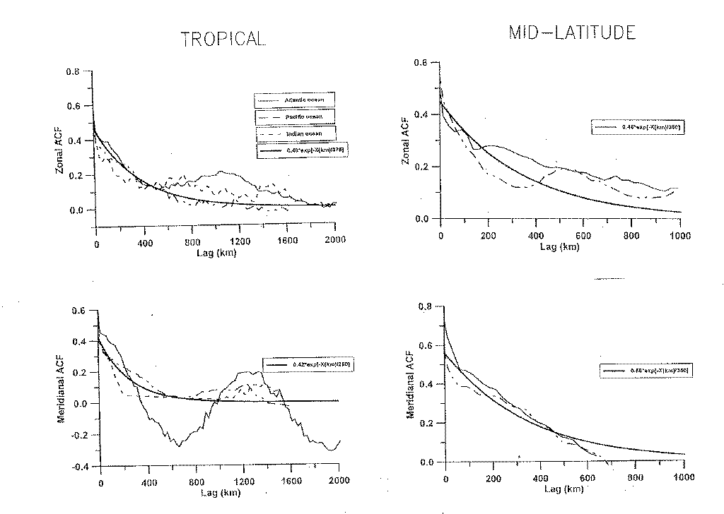
The zonal and meridional lagged autocorrelation
functions for temperature error at 75 m in the tropical and midlatitude
domains are shown in Fig. 3a-d. In
addition to the observed correlations for each basin the panels include
a correlation model. Assuming that the bias has been estimated correctly,
the error at zero lag provides an estimate of the normalized observation
error covariance ![]() . These values
are typically around 0.5. The spatial scales of the correlations all remain
in the range of 250-375 km at this depth, with the largest lags in the
zonal correlation in the tropics. These scales are similar to those proposed
by Meyers et al. (1991) based
on XBT data in the Pacific.
. These values
are typically around 0.5. The spatial scales of the correlations all remain
in the range of 250-375 km at this depth, with the largest lags in the
zonal correlation in the tropics. These scales are similar to those proposed
by Meyers et al. (1991) based
on XBT data in the Pacific.
A striking feature of the meridional autocorrelation in the tropics is a strong oscillatory pattern with a wavelength of 1200km in the tropical Atlantic (Fig. 3c). We have examined the cause of this pattern and found it to be the result of the ridge-trough system of thermocline undulations associated with the zonal equatorial currents. When one current is altered the others are affected.
After fitting exponential curves to each
of the spatial covariances, we construct an analytic form for the dependence
of ![]() and
and ![]() on
depth and latitude as:
on
depth and latitude as:
 ,
(7a)
,
(7a)
 .
(7b)
.
(7b)
The time-scale of the autocovariance of
observation minus forecast differences was similarly estimated to be ![]() .
The vertical covariance function of unbiased forecast error is particularly
inhomogeneous. This quantity is very large in the mixed layer and of the
scale of the pycnocline at pycnocline depths.
.
The vertical covariance function of unbiased forecast error is particularly
inhomogeneous. This quantity is very large in the mixed layer and of the
scale of the pycnocline at pycnocline depths.
After completing the analysis it makes
sense, as Smith (1995) suggests,
to go back and check the assumptions on which our analysis is based.
Daley (1992) has suggested examining the temporal correlation of
the observation minus forecast differences. Improvements in the analysis
system should be reflected in reductions in the temporal (and spatial)
scales of correlation. Alternatively, Hollingsworth
and Lonnberg (1989) have proposed examination of the observation
minus analysis differences. In principle, these latter differences should
be uncorrelated. Any spatial correlation in these differences represents
information that has not been extracted by the analysis. Here we follow
Hollingsworth and Lonnberg and examine the observation
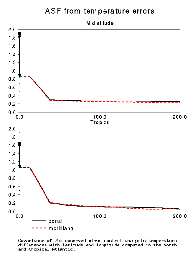
minus analysis differences. The 75m temperature differences were binned
into small ![]() bins in the same
regions as used in deriving (7). The variance of observed minus forecast
temperature in the tropical Atlantic is
bins in the same
regions as used in deriving (7). The variance of observed minus forecast
temperature in the tropical Atlantic is ![]() (Fig.
4). The covariance at lags between 25 and 50 km is less than
(Fig.
4). The covariance at lags between 25 and 50 km is less than ![]() .
.
We now discuss the structure of the covariance
![]() in (7). In the simple case
where the variables
in (7). In the simple case
where the variables ![]() and
and ![]() represent
forecast temperature errors at two locations
represent
forecast temperature errors at two locations ![]() is
simply the product of the unbiased forecast error standard deviations at
two locations
is
simply the product of the unbiased forecast error standard deviations at
two locations![]() . We anticipate
a close relationship between temperature and salinity errors at pycnocline
depths in many parts of the ocean (the importance of the temperature-salinity
relationship to the assimilation problem is discussed in Cooper
and Hanes, 1996). However, the relationship varies with location
because of the varying distribution of water masses. Here we use our CTD
data set to construct a lookup table for the temperature-salinity error
covariance as a function of
. We anticipate
a close relationship between temperature and salinity errors at pycnocline
depths in many parts of the ocean (the importance of the temperature-salinity
relationship to the assimilation problem is discussed in Cooper
and Hanes, 1996). However, the relationship varies with location
because of the varying distribution of water masses. Here we use our CTD
data set to construct a lookup table for the temperature-salinity error
covariance as a function of ![]() .
Among the difficulties encountered in constructing this table is the necessity
of excluding the high latitude regions of the northern ocean where the
relationship between temperature and salinity error is multiply-valued.
.
Among the difficulties encountered in constructing this table is the necessity
of excluding the high latitude regions of the northern ocean where the
relationship between temperature and salinity error is multiply-valued.
One of the most extensive data sets used
in our assimilation analysis is altimeter-derived sea level. Here we follow
the reasoning of Carton et al. (1996). We anticipate
that sea level and density forecast errors are negatively correlated because
of the tendency of the ocean to compensate for a rise of sea level with
a depression of the pycnocline. This assumption together with the assumption
that the variations in sea level are "small" leads to the conclusion
that for sea level error and temperature error ![]() should be approximately proportional to the mean vertical temperature gradient
( -
should be approximately proportional to the mean vertical temperature gradient
( -![]() ). In this formula
). In this formula ![]() is
an empirical nondimensional constant which determines the amplitude of
isopycnal depth displacement error implied by sea level error. Based on
comparison of the TOGA/TAO thermistor data and TOPEX/Poseidon altimetry
Carton et al. show that
is
an empirical nondimensional constant which determines the amplitude of
isopycnal depth displacement error implied by sea level error. Based on
comparison of the TOGA/TAO thermistor data and TOPEX/Poseidon altimetry
Carton et al. show that ![]() should
lie in a range of 100-200 in the tropical Pacific (a +1 cm sea level forecast
error implies a -1 to -2m isopycnal depth error). For the current study
we have recalculated
should
lie in a range of 100-200 in the tropical Pacific (a +1 cm sea level forecast
error implies a -1 to -2m isopycnal depth error). For the current study
we have recalculated ![]() based
on the global historical sea level and isopycnal depth variations obtained
from a preliminary assimilation analysis. Similarly, the relationship between
forecast salinity error and sea level error is proportional to the mean
vertical salinity gradient ( -
based
on the global historical sea level and isopycnal depth variations obtained
from a preliminary assimilation analysis. Similarly, the relationship between
forecast salinity error and sea level error is proportional to the mean
vertical salinity gradient ( -![]() ).
Error in the analysis salinity typically contributes 1-2 cm to the observed
sea level error.
).
Error in the analysis salinity typically contributes 1-2 cm to the observed
sea level error.
Because the detailed structure of earth's geoid is uncertain, the sea level estimates from Geosat and those of later overlapping missions (ERS1 and TOPEX/Poseidon) each differ from 'true sea level' by an unknown stationary, but spatially varying mean. In this study we compensate for these two unknown means by removing time-mean sea level from the data sets and replacing them with time mean sea level produced by an experimental analysis in which altimetry was not assimilated, and computed for the same period as each mission. In this way, the effect of the altimetry in the time-mean sea level is minimized, while still contributing to the trend, and to shorter time-scale variability.
The procedure for updating temperature
errors in the mixed layer is somewhat different than for subsurface errors.
The reason for this distinction is the availability of a more extensive
data set, and the fact that the mixed layer has broader spatial scales,
and stronger vertical coherence. At the update time step the forecast depth
of the mixed layer is the depth at which forecast density has increased
from its surface value by ![]() .
This value was chosen as the result of a series of experiments and depends
on the model resolution and mixing parameterization. The sea surface temperature
provided by Reynolds and Smith (1994), itself
the result of objectively combining satellite, shipboard, and buoy sea
surface temperature observations, is used as an estimate of mixed layer
temperature. Sea surface salinity currently is relaxed to its climatological
seasonal value in this layer (temperature and salinity errors are assumed
to be uncorrelated within the mixed layer).
.
This value was chosen as the result of a series of experiments and depends
on the model resolution and mixing parameterization. The sea surface temperature
provided by Reynolds and Smith (1994), itself
the result of objectively combining satellite, shipboard, and buoy sea
surface temperature observations, is used as an estimate of mixed layer
temperature. Sea surface salinity currently is relaxed to its climatological
seasonal value in this layer (temperature and salinity errors are assumed
to be uncorrelated within the mixed layer).
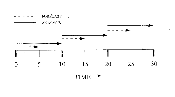
Time-stepping in the analysis is carried out using the incremental update analysis method of Bloom (1996). In this approach, illustrated in Fig. 5 , we begin with a preliminary 5-day forecast (dashed line). At day 5 the forecast error is estimated using the procedure outlined above. Then we go back and carry out a 10-day integration starting from day 0, correcting the mass fields for the estimated forecast error (solid line). This corrected integration is our analysis. The analysis at day 10 provides initial conditions for the next 5-day preliminary forecast. The forecast error is computed on day 15, then we go back and carry out a new 10-day analysis beginning on day 10 and the cycle repeats itself. This predictor-corrector time-stepping method has two advantages. The first is that it acts like a continuous assimilation method by keeping the mass and momentum fields in balance, thus suppressing gravity waves otherwise expected to be produced by the updating procedure. The second is that it reduces the impact of bias on the analysis by 50% because the forecast is continually corrected for the estimated forecast error, which includes an estimate of the remaining bias. The cost of this procedure is a 50% increase in the integration time of the model forecast over that of a simple 10-day intermittent analysis.
The assimilation procedure relies on the
forecast of an ocean model based on the Geophysical Fluid Dynamics Laboratory
Modular Ocean Model 2.2 software. The model horizontal resolution is ![]() in
the tropics, expanding to a uniform
in
the tropics, expanding to a uniform ![]() resolution
at midlatitude. The basin domain extends from
resolution
at midlatitude. The basin domain extends from ![]() to
to ![]() for a total of
for a total of ![]() horizontal grid points. At the polar boundaries the temperature and salinity
fields relaxed to climatology. We make no attempt to model cryospheric
or deepwater formation processes explicitly. A weak 5-year relaxation of
the global temperature and salinity fields is included in order to reduce
forecast bias in deep water masses. Bottom topography is included. The
model has 20 levels in the vertical, with 15m resolution in the upper 150m.
The time step is 1 hr. The resolution was chosen to be as high as possible
while still allowing experiments to be carried out on workstations. A 50-year
analysis currently requires three weeks on a Digital alpha workstation
with a 333 MHz CPU.
horizontal grid points. At the polar boundaries the temperature and salinity
fields relaxed to climatology. We make no attempt to model cryospheric
or deepwater formation processes explicitly. A weak 5-year relaxation of
the global temperature and salinity fields is included in order to reduce
forecast bias in deep water masses. Bottom topography is included. The
model has 20 levels in the vertical, with 15m resolution in the upper 150m.
The time step is 1 hr. The resolution was chosen to be as high as possible
while still allowing experiments to be carried out on workstations. A 50-year
analysis currently requires three weeks on a Digital alpha workstation
with a 333 MHz CPU.
For the period 1950-1992 the winds are provided by an historical analysis of Comprehensive Ocean/Atmosphere Data Set (COADS) surface wind observations by da Silva et al. (1994). Evidence suggests that the wind field contains erroneous long-term trends. Because of our concern we have removed a linear trend from both components of wind at each gridpoint. The impact of removing the trend is examined below. In order to allow us to extend the analysis past 1992, we have added to the wind record using National Center for Environmental Prediction (NCEP) winds for 1992-1995. The mean strength of the COADS and NCEP winds are different. In order to reduce changes in the analysis due to changes in the wind field we have corrected the NCEP winds to the mean of the COADS winds based on comparing the mean winds of the two historical analyses during a two-year period of overlap. Surface heat flux is effectively determined by surface temperature observations. Sea surface salinity is relaxed to climatological monthly salinity in this study.
3.2 Data impact
The first issue we address is the relative
importance of winds versus subsurface updating in contributing to the interannual
and decadal variability of the analysis. Variability is introduced into
the analysis either through inaccuracies in the forecast model and its
associated initial/boundary conditions, or through the updating procedure
and its associated suite of observations. In Expt.
2 (see Table 1) the control
analysis is repeated except without any subsurface updating (a simulation).
In this experiment interannual and decadal variability is due primarily
to variability in the historical wind field and SST. Thus, the difference
between Expt. 2 heat content and
heat content from the control analysis indicates the impact of the subsurface
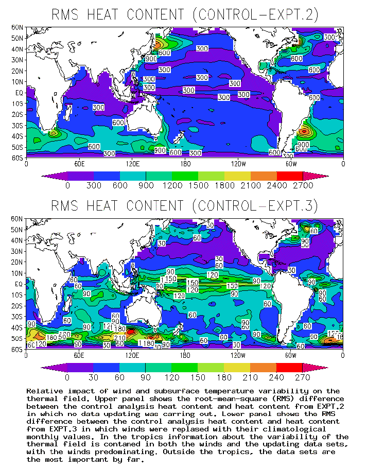
observations (Fig. 6, upper panel).
The subsurface observations have an impact throughout the basin exceeding
![]() in most places.
in most places.
In Expt.
3 the control analysis is repeated except that the winds are replaced
with their climatological monthly average. In this experiment interannual
and decadal variability is due to variability in the updating data sets.
Thus, the difference between Expt. 3
and the control analysis heat content is the result of the winds (Fig.
6, lower panel). The contribution of the winds is generally less
than ![]() except in the tropics
and the Circumpolar Current. Comparison of these results suggests the subsurface
data contain most of the information about changes in the subsurface thermal
field on interannual and longer time scales. In the tropics, though, winds
do contribute significantly.
except in the tropics
and the Circumpolar Current. Comparison of these results suggests the subsurface
data contain most of the information about changes in the subsurface thermal
field on interannual and longer time scales. In the tropics, though, winds
do contribute significantly.
We next consider the source of the long-term
trend in heat content. Recent studies by Clarke and Lebedev,
(1996) have shown that the trend in the historical wind field is
not matched by a trend in surface pressure, and thus is likely to be spurious.
Our response to this result has been to remove the long-term trend from
the wind field in most of our experiments. We examine the impact of removing
the wind trend by comparing the trend in heat content from Expt.
4 in which the wind field has not been detrended with the trend
in heat content from the control analysis (Fig.
7). The linear trend of heat content in the control analysis is
small, generally less than ![]() with the largest trends at high latitudes. In the subtropics heat content
has been rising by a more modest
with the largest trends at high latitudes. In the subtropics heat content
has been rising by a more modest ![]() ,
while in the tropics the trend has been toward cooling at a rate of -
,
while in the tropics the trend has been toward cooling at a rate of -![]() .
When the wind field trend is retained (Expt.
4 ) the heat content trend in the tropics increases by a factor
of 2 or more with strong cooling in the eastern tropics and warming in
the west as the result of the strengthening of the trade winds with time.
.
When the wind field trend is retained (Expt.
4 ) the heat content trend in the tropics increases by a factor
of 2 or more with strong cooling in the eastern tropics and warming in
the west as the result of the strengthening of the trade winds with time.
4. Global statistic
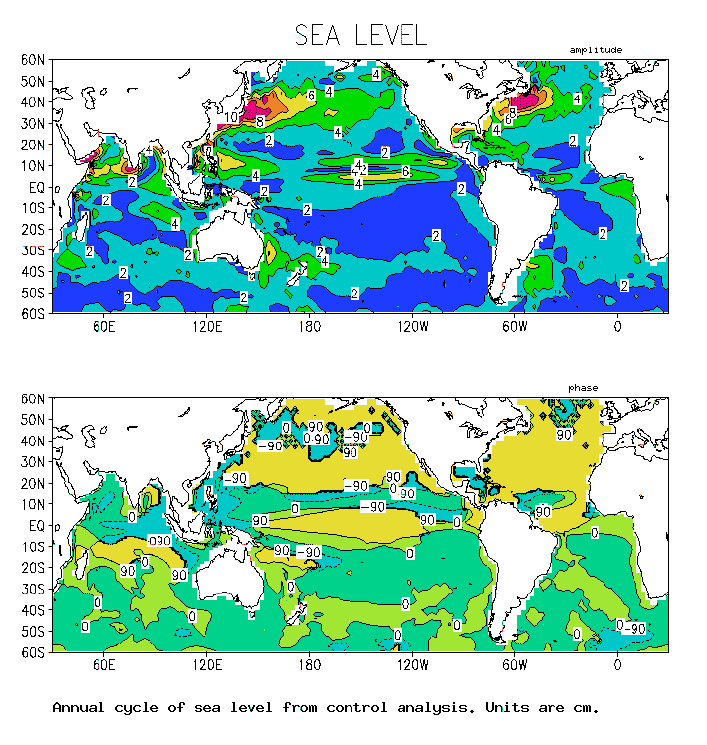
The strongest signal in the mass and momentum
fields is the annual shift of heat and mass in response to shifting winds
and surface heat flux. We introduce our control analysis by discussing
the annual cycle of two key quantities, sea level, and kinetic energy ![]() ,
based on the 46-year control analysis (Fig.
8a,b). A third variable, heat content,
will be discussed separately. The basin-scale structure of the annual cycle
of sea level is dominated by a pattern of rising level in the summer hemisphere
as a result of the antisymmetry about the equator of winds and solar heating.
Smaller scale variations are also evident. Western boundary current regions
of the North Atlantic and North Pacific have seasonal amplitudes approaching
15 cm (these results closely resemble those computed from short 1yr-long
altimeter records by Cheney et al, 1994). The
tropics also have distinct smaller-scale features. The tropical Atlantic
and Pacific show 4-6 cm variations in zonal bands resulting from seasonal
changes in the North Equatorial Countercurrent. The corresponding amplitude
of heat content in these regions (not shown) is
,
based on the 46-year control analysis (Fig.
8a,b). A third variable, heat content,
will be discussed separately. The basin-scale structure of the annual cycle
of sea level is dominated by a pattern of rising level in the summer hemisphere
as a result of the antisymmetry about the equator of winds and solar heating.
Smaller scale variations are also evident. Western boundary current regions
of the North Atlantic and North Pacific have seasonal amplitudes approaching
15 cm (these results closely resemble those computed from short 1yr-long
altimeter records by Cheney et al, 1994). The
tropics also have distinct smaller-scale features. The tropical Atlantic
and Pacific show 4-6 cm variations in zonal bands resulting from seasonal
changes in the North Equatorial Countercurrent. The corresponding amplitude
of heat content in these regions (not shown) is ![]() .
.
In contrast to sea level and heat content,
the annual cycle of kinetic energy (Fig.
8b) is largest in tropics, reflecting the seasonal changes in the
tropical current system. The annual amplitude of these currents exceeds
20 cm/s. In the tropical Pacific the intensity of the current is reduced
somewhat near ![]() . The annual kinetic
energy in the Indian Ocean is elevated throughout, with highest values
along the western boundary in the region of the seasonal Somali Current.
. The annual kinetic
energy in the Indian Ocean is elevated throughout, with highest values
along the western boundary in the region of the seasonal Somali Current.
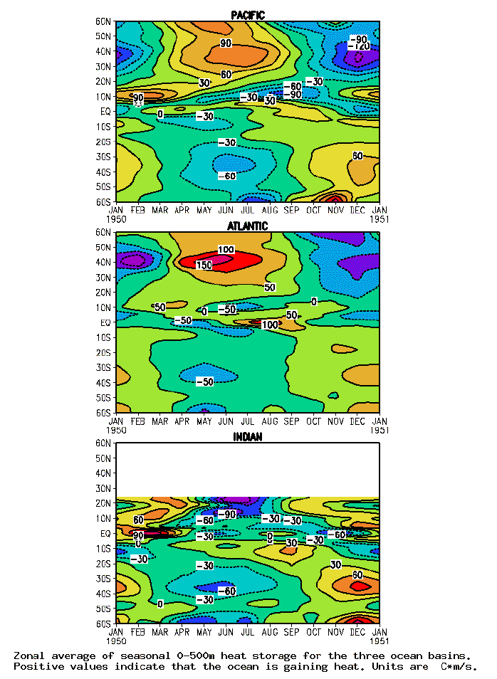
Seasonal variations in local heat storage
reflect the difference between net surface heating and horizontal divergence
of heat transport. Because the ocean basins are bounded to the east and
west at most latitudes, the zonal average of heat storage, shown in Fig.
9a-c for the three basins, is the difference between net surface
heating and the meridional divergence of heat transport. Here storage is
computed by taking the center difference from successive monthly averages.
These results can be directly compared with the results of Hsiung
et al. (1989). Heat storage in the Pacific follows the cycle of
solar radiation with a maximum in the Northern Hemisphere in June-August.
The seasonal maximum is somewhat lower than in the previous study. Maximum
heat loss from the Southern Hemisphere occurs perhaps a few weeks earlier.
The pattern of heat storage near the equator is more complex, and was not
well resolved in the earlier study. The period July-October is one in which
the region from ![]() is storing
heat rapidly as a result of the appearance of the cold tongue in the eastern
Pacific, while the region from
is storing
heat rapidly as a result of the appearance of the cold tongue in the eastern
Pacific, while the region from ![]() is losing heat rapidly.
is losing heat rapidly.
Heat storage in the Atlantic generally
resembles heat storage in the Pacific (Fig.
9b). In the Atlantic maximum heat storage occurs somewhat earlier
(May-July). Rapid heat storage along and south of the equator is limited
to the months July-September. North of the equator heat is being exported
mainly during early boreal summer. Heat storage in the tropical Indian
Ocean (Fig. 9c) is quite complicated.
Between ![]() the southern Indian
Ocean is gaining heat during June-October, a period in which the Sun is
actually in the Northern Hemisphere. This region is losing heat during
November-March, a period in which the Sun has crossed over into the Southern
Hemisphere! These counterintuitive results are consistent with those of
Hsiung et al. (1989).
the southern Indian
Ocean is gaining heat during June-October, a period in which the Sun is
actually in the Northern Hemisphere. This region is losing heat during
November-March, a period in which the Sun has crossed over into the Southern
Hemisphere! These counterintuitive results are consistent with those of
Hsiung et al. (1989).
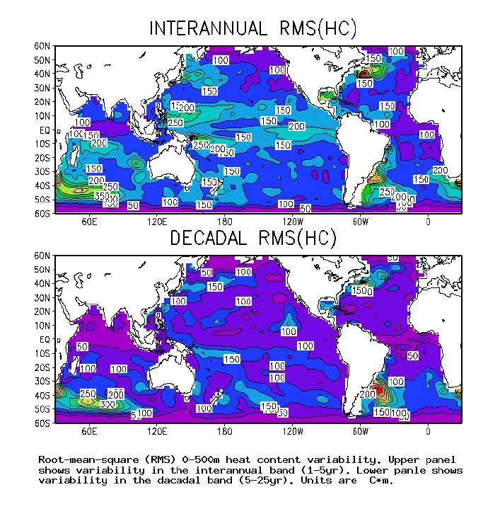
At periods longer than the annual cycle the distribution of variance changes. In Fig. 10 we present a crude decomposition of the spectral characteristics of the heat content field by separating the heat content variability into the interannual band (1-5 yr) and the decadal band (5-25 yr). At interannual periods the variability along the equator in the Pacific is enhanced and shifted eastward, while off-equatorial variability occurs in the western side of the basin. The western tropical Indian Ocean has significant variability, as do the eddy production regions of the western boundary currents and Circumpolar Current. At decadal periods the tropics become less prominent relative to the subtropical and midlatitude gyres. The shift of variability from the tropics toward midlatitude as the frequency decreases reflects the fundamental dynamical properties of the ocean.
Much of the heat content variability at
interannual and decadal periods in Fig.
10 is spatially incoherent. In order to explore the sources of
just that part of the heat content signal which has basin-scales we define
three focal areas, one in the central North Pacific (averaged, ![]() ),
a second in the eastern tropical Pacific (averaged
),
a second in the eastern tropical Pacific (averaged ![]() ),
and a third in the central North Atlantic (averaged
),
and a third in the central North Atlantic (averaged ![]() ).
Note that the focal area in the North Atlantic is smaller than the others,
reflecting the smaller spatial scales of variability there. The time series
of area-averaged heat content anomaly are presented in Fig.
11 (a linear trend has been removed, consistent with the previous
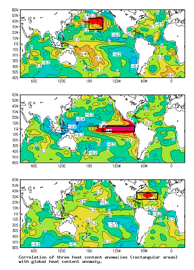
analysis). In order to define the spatial structure of these modes we correlate
the three heat content anomaly time-series with heat content anomaly throughout
the global ocean. The three resulting correlation maps are shown in Fig.
12.
).
Note that the focal area in the North Atlantic is smaller than the others,
reflecting the smaller spatial scales of variability there. The time series
of area-averaged heat content anomaly are presented in Fig.
11 (a linear trend has been removed, consistent with the previous
analysis). In order to define the spatial structure of these modes we correlate
the three heat content anomaly time-series with heat content anomaly throughout
the global ocean. The three resulting correlation maps are shown in Fig.
12.
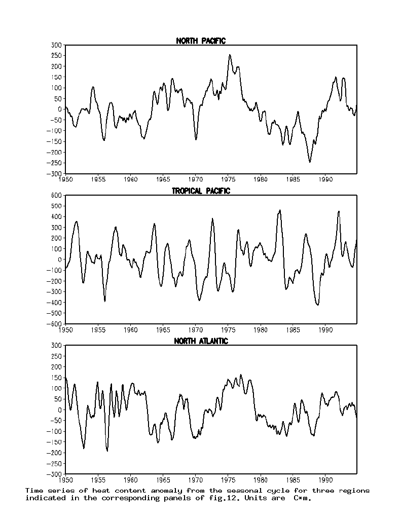
The time series and spatial pattern of correlation with North Pacific heat content is shown in the upper panels of Figs. 11 and 12. The variability is substantially decadal. The most prominent feature of the time series is a cooling during the 1980s following a relatively warm 1970s. Heat content variability in the North Pacific has been related to fluctuations in the Pacific-North-America pattern of wind variation (Trenberth and Hurrell, 1994; Graham, 1994). Changes in the wind patterns in 1976-1977 led to a cooling in the central basin which was referred to as a climate shift by Miller et al. (1994). This climate shift is evident in Fig. 11, but is followed 11 years later by a return to warm conditions, also noted by Levitus and Antonov (1995).
By correlating the North Pacific time series with heat content anomaly time series for the rest of the oceans we can identify the spatial pattern of oceanic thermal variability. The region that is most highly correlated with the midlatitude North Pacific, interestingly, is the western tropical and southern Pacific. Much of the correlation results from a drop in heat content in the 1970s that approximately coincides with the drop in the central North Pacific. Between these two regions heat content is a region of negative correlation. This pattern of alternating positive and negative correlation is reminiscent of ideas of a slow advection of thermal anomalies throughout the North Pacific (e.g. Latif and Barnett, 1994; Deser et al., 1996).
Next we turn our attention to the tropical
Pacific. The variability here is strongly interannual, reflecting the importance
of El ![]() Oscillation. Individual
peaks in the time series can be identified with individual
Oscillation. Individual
peaks in the time series can be identified with individual![]() .
Examination of the time series shows that the amplitude and frequency of
heat content variability has been fairly regular during the past five decades,
without major interruptions. Decadal variability is also evident in the
time series. The late-1970s were a period of gradual warming coinciding
with a warming of SST (Wang, 1995).
.
Examination of the time series shows that the amplitude and frequency of
heat content variability has been fairly regular during the past five decades,
without major interruptions. Decadal variability is also evident in the
time series. The late-1970s were a period of gradual warming coinciding
with a warming of SST (Wang, 1995).
Examination of the spatial pattern of correlation
with tropical Pacific heat content shows the spatial structure of the oceanic
expression of El ![]() Oscillation.
For example, we find that on either side of the zonal band of high correlation
near the equator are bands of negative correlation. The band of negative
correlation in the Northern Hemisphere is most coherent, extending west-southwestward
from the west coast of North America. The existence of off-equatorial bands
of negative correlation are a key feature of the delayed-oscillator theories
of the periodicity of El
Oscillation.
For example, we find that on either side of the zonal band of high correlation
near the equator are bands of negative correlation. The band of negative
correlation in the Northern Hemisphere is most coherent, extending west-southwestward
from the west coast of North America. The existence of off-equatorial bands
of negative correlation are a key feature of the delayed-oscillator theories
of the periodicity of El ![]() Oscillation.
The zone of negative correlation extends into the eastern Indian Ocean,
suggesting a connection between the western Pacific and Eastern Indian
Ocean. Examination of the lagged correlation shows that the band of positive
correlation near the equator shifts eastward and poleward when the time
lag is increased to a few months, while the off-equatorial bands of negative
correlation shift westward.
Oscillation.
The zone of negative correlation extends into the eastern Indian Ocean,
suggesting a connection between the western Pacific and Eastern Indian
Ocean. Examination of the lagged correlation shows that the band of positive
correlation near the equator shifts eastward and poleward when the time
lag is increased to a few months, while the off-equatorial bands of negative
correlation shift westward.
The impact of El ![]() Oscillation
on the North and tropical Atlantic has been examine in a number of studies
(e.g. Carton and Huang, 1994; Enfield
and Meyer, 1994). In the tropical Atlantic Carton
and Huang have proposed that the changes in western tropical Atlantic
winds associated with warm SST in the eastern tropical Pacific leads to
a buildup of heat in the western tropical Atlantic. This anomalous heat,
which occurs on the form of anomalous deepening of the thermocline, eventually
leads to a deepening of the equatorial thermocline and contributes to warming
in the eastern Atlantic. Some confirmation for these ideas is apparent
in the weakly positive correlation (0.2) between eastern tropical Pacific
heat content and western tropical Atlantic
heat content. The final time series in the lower panel of Fig.
11 represents the central North Atlantic Ocean. Heat content variability
in the North Atlantic is also associated with variability in the sector
winds, in this case the North Atlantic Oscillation pattern Atlantic winds
(Hurrell and Van Loon, 1997). The time series
of heat content shows rich decadal variability. The 1950s are relatively
warm, followed by a series of cool events in the early 1960s, the late-1960s
and early 1970s, and again in the late-1970s and early 1980s. The second
of these cool events has been documented by S. Levitus (Levitus,
1989, 1990).
Oscillation
on the North and tropical Atlantic has been examine in a number of studies
(e.g. Carton and Huang, 1994; Enfield
and Meyer, 1994). In the tropical Atlantic Carton
and Huang have proposed that the changes in western tropical Atlantic
winds associated with warm SST in the eastern tropical Pacific leads to
a buildup of heat in the western tropical Atlantic. This anomalous heat,
which occurs on the form of anomalous deepening of the thermocline, eventually
leads to a deepening of the equatorial thermocline and contributes to warming
in the eastern Atlantic. Some confirmation for these ideas is apparent
in the weakly positive correlation (0.2) between eastern tropical Pacific
heat content and western tropical Atlantic
heat content. The final time series in the lower panel of Fig.
11 represents the central North Atlantic Ocean. Heat content variability
in the North Atlantic is also associated with variability in the sector
winds, in this case the North Atlantic Oscillation pattern Atlantic winds
(Hurrell and Van Loon, 1997). The time series
of heat content shows rich decadal variability. The 1950s are relatively
warm, followed by a series of cool events in the early 1960s, the late-1960s
and early 1970s, and again in the late-1970s and early 1980s. The second
of these cool events has been documented by S. Levitus (Levitus,
1989, 1990).
5. Conclusions
Here we present a description of the Simple Ocean Data Assimilation (SODA) package. The package contains all components of an analysis system that we can anticipate in the future, including an ocean general circulation model, models of the observation and forecast error, the basic hydrographic, altimeter, and SST data sets, and a constraint algorithm. Particular attention is focused on the problem of bias in the model forecast and its effects on the analysis. We use SODA to construct a retrospective analysis of temperature, salinity, and current in the upper layers of the ocean globally during the past five decades.
Our examination of the analysis is presented in two parts. In Carton et al. (1998) we present a series of direct comparisons to independent observations, including tide gauge sea level, World Oceanographic Circulation Experiment hydrographic sections, ocean weather station time series, surface drifters, and moored currents. The major deficiencies are bias in the forecast model, inadequacies in the surface freshwater budget, the lack of resolution of important topographic features, and problems with sufficient water mass production in the subtropics and tropics. We feel that the treatment of the mixed layer needs to take into account more completely than we have done, the distinct physical processes occurring there. Still, despite these limitations the analysis bears appealing similarity to the independent observations.
However, to be useful for climate studies the analysis should contain realistic basin-scale modes of variability. In the current study we explore the analysis from the point of view of searching for these basin-scale modes. At the annual period both hemispheres show a strong response to seasonal forcing of surface winds, heat and freshwater. In the subtropics and midlatitudes sea level varies in phase with seasonal changes in solar radiation, except in the southern Indian Ocean. Closer to the equator the phase of sea level undergoes rapid reversals as the ocean responds to strong annual variations in winds.
Heat content variability at interannual
periods (1 - 5 yr) is similar in size to the variability at the annual
period. The strongest basin-scale signal is associated with El ![]() Oscillation.
To explore this pattern of variability we examine the correlation of global
heat content with the heat content time series from a region of the eastern
equatorial Pacific (the Nino3 region) that is itself considered an index
of El
Oscillation.
To explore this pattern of variability we examine the correlation of global
heat content with the heat content time series from a region of the eastern
equatorial Pacific (the Nino3 region) that is itself considered an index
of El ![]() Oscillation. Our examination
of the zero lag correlation of global heat content shows the eastern and
western tropical Pacific to be out of phase. The correlation between the
two ranges between -0.4 and -0.6. The eastern Indian Ocean is in phase
with the western Pacific and thus is out of phase with the eastern Pacific.
The subtropics are also out of phase with the eastern Pacific, although
the strength of the correlation is lower. When eastern equatorial Pacific
heat content time series leads by 6 months the pattern of correlation along
the Pacific equator shifts eastward and the pattern of correlation in the
Pacific subtropics shifts westward. The North Pacific has a weak positive
correlation with the eastern equatorial Pacific. Correlations between eastern
Pacific heat content and Atlantic heat content are modest.
Oscillation. Our examination
of the zero lag correlation of global heat content shows the eastern and
western tropical Pacific to be out of phase. The correlation between the
two ranges between -0.4 and -0.6. The eastern Indian Ocean is in phase
with the western Pacific and thus is out of phase with the eastern Pacific.
The subtropics are also out of phase with the eastern Pacific, although
the strength of the correlation is lower. When eastern equatorial Pacific
heat content time series leads by 6 months the pattern of correlation along
the Pacific equator shifts eastward and the pattern of correlation in the
Pacific subtropics shifts westward. The North Pacific has a weak positive
correlation with the eastern equatorial Pacific. Correlations between eastern
Pacific heat content and Atlantic heat content are modest.
At longer decadal periods (5 - 25 yr) the variability in the analysis decreases somewhat. We search for heat content variations that are correlated with heat content in the central North Pacific and for heat content variations that are correlated with heat content in the central North Atlantic. The global influences of the Pacific-North America wind pattern leads to broad patterns of correlation in heat content variability with variability in the central North Pacific. Increases in heat content in the central North Pacific are associated with decreases in heat storage in the subtropical Pacific and increases in the western tropical Pacific. Atlantic heat content is positively correlated in general with the central North Pacific. The relationship is confirmed by correlating the heat content anomaly in the central North Atlantic with global heat content.
Acknowledgments
We are grateful to a number of people who have given us access to their data sets. Mark Swenson and Zengxi Zhou of the Atlantic Oceanographic Marine Laboratory/NOAA have provided the monthly-averaged surface drifters, Sydney Levitus, and Robert Cheney and their colleagues at the National Oceanographic Data Center/NOAA have given us access to the hydrographic and altimeter data. We have benefited from the data sets collected by Principal Investigators of the Tropical Ocean/global Atmosphere and World Oceanographic Circulation Experiments. We thank Dick Dee and Arlindo da Silva of the Data Assimilation Office/NASA for many discussions on the subject of data assimilation. Finally, we want to express our gratitude for support from the Office of Global Programs/NOAA under grants (NA66GP0269 to JAC) and (NA76GP0559 to BSG), and the National Science Foundation under grant (OCE9416894 to JAC).
References
Bennett, A.F., 1990: Inverse methods in physical oceanography. Cambridge University Press, New York, 346pp.
Bloom, S.C. 1996: Data assimilation using incremental analysis updates. Mon. Wea. Rev., 124, 1256-1271.
Carton, J.A., B.S. Giese, X. Cao, and L. Miller, 1996: Impact of altimeter, thermistor, and expendable bathythermograph data on retrospective analyses of the tropical Pacific Ocean, J. Geophys. Res., 101, 14, 147-14159.
Carton, J.A. , G. Chepurin, and X. Cao, 1998: A retrospective analysis of the global ocean 1950-1995 and its comparison to observations. Submitted.
Carton, J.A., and B. Huang, 1994: Warm events in the tropical Atlantic, J. Phys. Oceanogr., 24, 888-903.
Cheney, R.E., L. Miller, and J. Lillibridge, 1994: Topex/Poseidon, the 2 cm solution. J. Geophys. Res., 99, 24,555-.
Clarke, A.J., and A. Lebedev, 1996: Long-term changes in the equatorial Pacific trade wind systems. J. Clim., 9, 1020-1028.
Cooper, A., and K. Haines, 1996: Data assimilation with water property conservation. J. Geophys. Res., 101, 1059-1077.
da Silva, A. M., C. C. Young and S. Levitus, 1994: Atlas of Surface Marine Data 1994, Volume 1: Algorithms and Procedures. NOAA Atlas NESDIS 6, U.S. Department of Commerce, NOAA, NESDIS.
Daley, R., 1991: Atmospheric data analysis. Cambridge University Press, NY, 457pp.
Daley, R., 1992: the lagged innovation covariance: A performance diagnostic for atmospheric data assimilation. Mon. Wea. Rev., 120, 178-196.
Dee, R., and A.M. da Silva, 1997: Data assimilation in the presence of forecast bias. Submitted to Q. J. R. Met. Soc.
Deser, C. Alexander, M. A., Timlin, M. S., 1996: Upper-ocean thermal variations in the North Pacific during 1970-1991. J. Clim., 9,1840- .
Enfield, D.B., and D.A.
Meyer, 1997: Tropical Atlantic sea surface temperature variability and
its relation to El ![]() Oscillation,
J. Geophys. Res., 102, 929-945.
Oscillation,
J. Geophys. Res., 102, 929-945.
Graham, N.E., 1994: Decadal-scale climate variability in the tropical and North Pacific during the 1970s and 1980s: observations and model results. Clim. Dynam., 10, 135-162.
Hollingsworth, A., and P. Lonnberg, 1989: the verification of objective analyses: diagnostics of analysis system performance. Meteorol. Atmos. Phys., 40, 3-27.
Hsiung, J., R.E. Newell, and T. Houghtby, 1989: The annual cycle of oceanic heat storage and oceanic meridional heat transport, Q. J. Roy. Met. Soc., 115, 1-28.
Hurrell, J.W., and H. Van Loon, 1997: decadal variations in climate associated with the North Atlantic Oscillation, Clim. Change, 36, 301-
Ji, M., A. Leetmaa, and J. Derber, 1995: An ocean analysis system for seasonal to interannual climate studies. Mon. Wea. Rev., 123, 460-481.
Latif, M. and T. Barnett, 1994: Causes of decadal climate variability over the North Pacific and North America, Science, 266, 634-637.
Levitus, S., 1989: Interpentadal variability of salinity in the upper 150 m of the North Atlantic Ocean Versus 1955-1959. J. Geophys. Res., 94, 9679-
Levitus, S., 1990: Interpentadal variability of steric sea level and geopotential thickness of the North Atlantic Ocean, 1970-1974 Versus 1955-1959. J. Geophys. Res., 95, 5233-
Levitus, S. and T. Boyer, 1994: World Ocean Atlas 1994, Vol. 4: Temperature, NESDIS, 117pp., Natl. Env. Satell. Data and Int. Serv., Natl. Oceanic and Atmos. Admin., Atlas series, Washington, D.C.
Levitus, S., T.P. Boyer, and J. Antonov, 1994: World Ocean Atlas, 1994, Vol.5: Interannual variability of upper ocean thermal structure, 176pp., Natl. Env. Satell. Data and Int. Serv., Natl. Oceanic and Atmos. Admin., Atlas series, Washington, D.C..
Levitus, S., and J. Antonov, 1995: Observational Evidence of Interannual to Decadal-Scale Variability of the Subsurface Temperature-Salinity Structure of the World Ocean. Climatic Change, 31, 495-.
Malanotte-Rizzoli, P., 1996: Modern Approaches to Data Assimilation in Ocean Modeling, Elsevier, New York, 455pp.
Meyers, G., H. Phillips, N. Smith, and J. Sprintall, 1991: space and timescales for optimal interpolation of temperature - tropical Pacific Ocean, Prog. Oceanogr., 28, 189-218.
Miller, A.J., Cayan, D. R., and T. P. Barnett, 1994: The 1976-77 Climate Shift of the Pacific Ocean. Oceanography, 7, 21-.
Reynolds, R.W. and T.M. Smith, 1994: Improved global sea surface temperature analysis using optimum interpolation. J. Clim., 7, 929-948.
Rosati, A., R. Gudgel, and K. Miyakoda, 1995: Decadal analysis produced from an ocean assimilation system. Mon. Wea. Rev., 123, 2,206-.
Smith, N.R., 1995: An improved system for tropical ocean subsurface temperature analysis. J. Atmos. And Ocean Tech., 12, 850-.
Thiebaux, H.J. and L.L. Morone, 1990: short-term systematic errors in global forecasts: their estimation and removal. Tellus, 42a, 209-229.
Trenberth, K.E., and J.W. Hurrell, 1994: Decadal atmosphere-ocean variations in the Pacific, Climate Dynam., 9, 303-319.
Wang, B., 1995: Interdecadal changes in El Nino onset in the last four decades. J. Clim., 8, 267-285.
White, W.B., 1995: Design of a global observing system for basin-scale upper ocean temperature anomalies. Prog. Oceanogr., 36, 169-217.
Wunsch, C., 1996: The ocean circulation inverse problem. Cambridge University Press, New York, 442pp.
Figure Legends
Fig. 1 a) Distribution of combined subsurface temperature observations at 75m with time. The dates of the recent altimeter satellites are indicated. b) Distribution of the combined subsurface temperature observations with latitude and longitude. Shading indicates density.
Fig. 2
Influence of bias on analysis. Sea level from control analysis ![]() and
Expt. 1 (
and
Expt. 1 (![]() )
in the central North Pacific (
)
in the central North Pacific (![]() ).
The average difference is 3.9cm.
).
The average difference is 3.9cm.
Fig. 3
Covariance of temperature observation error with zonal and meridional
lag for three ocean basins. a) Zonal tropical, b) zonal midlatitude, c)
meridional tropical, and d) meridional midlatitude. The vertical axis is
![]() . Solid curves show
model covariance. Vertical line at zero lag indicates the size of the observation
error covariance.
. Solid curves show
model covariance. Vertical line at zero lag indicates the size of the observation
error covariance.
Fig. 4 Covariance of 75m observed minus forecast temperature differences with latitude and longitude computed in the North and tropical Atlantic.
Fig. 5 Illustration of the incremental update analysis procedure of Bloom (1996). Preliminary 5-day forecasts are indicated with dashed lines. The first forecast begins on day 0. At day 5 forecast errors are estimated. A second 10-day forecast is carried out starting from day 0 (solid line). In this forecast the mass fields are continuously corrected for the estimated forecast error. The analysis at day 10 provides initial conditions for the next 5-day preliminary forecast. The procedure repeats itself every 10 days.
Fig. 6 Relative impact of wind and subsurface temperature variability on the thermal field. Upper panel shows the root-mean-square difference between the control analysis heat content and heat content from Expt. 2 in which no data updating is carried out. Lower panel shows the root-mean-square difference between the control analysis heat content and heat content from Expt. 3 in which winds are replaced with their climatological monthly values. In the tropics information about the interannual variability of the thermal field is contained in both the winds and the updating data sets, with the winds predominating. Outside the tropics, the updating data sets are the most important by far.
Fig. 7
Contribution of trends in the winds to trends in subsurface temperature.
Upper panel shows the trend of 0/500m heat content at each point computed
using the full 46-year record for Expt. 4
in which the wind field was not detrended. Striking changes occur
along the equator. In the Atlantic and Pacific the intensification of the
trade winds with time leads to a gradual intensification of the zonal gradient
of heat storage. Lower panel shows a similar map of heat content trend
for the control analysis for which a linear trend was removed from the
winds. Units are ![]() .
.
Fig. 8 Annual cycle of a)
kinetic energy, and b) sea level from the
control analysis. Sea level has strong amplitude in the high variability
regions of the western boundary current. The maximum amplitude in these
regions approaches 15 cm. Units are ![]() ,
,
![]() , and cm.
, and cm.
Fig. 9
Zonal average of seasonal 0/500 m heat storage for the three ocean basins.
Positive values indicate that the ocean is gaining heat. Units are ![]() .
.
Fig. 10
Root-mean-square 0/500 m heat content variability. (a) in the interannual
band (1-5 yr), (b) decadal band (5-25 yr). Units are ![]() .
.
Fig. 11
Time series of heat content anomaly from the seasonal cycle for three regions,
a) North Pacific (averaged, ![]() ),
b) Nino3 region of the eastern tropical Pacific (averaged
),
b) Nino3 region of the eastern tropical Pacific (averaged ![]() ),
and c) North Atlantic (averaged
),
and c) North Atlantic (averaged ![]() ).
The regions are indicated in the corresponding panels of Fig.
12. Units are
).
The regions are indicated in the corresponding panels of Fig.
12. Units are ![]() .
.
Fig. 12 Correlation of three heat content anomaly time series shown in Fig. 11 with global heat content anomaly. a) North Pacific, b) tropical Pacific, and c) North Atlantic.